The debt market plays a vital role in the economy, and understanding how debt securities respond to changes in interest rates is crucial for navigating this market effectively. To start, it’s essential to clarify some key definitions. First, a bond is a type of debt security where an investor loans money to an issuer, typically a corporation or government entity, in exchange for regular interest payments and the return on their principal investment.
At its core, a bond represents a loan from the investor to the issuer. “Fixed income” refers to the regular, predictable income earned from investing in bonds and other debt securities, which typically offer a fixed rate of return over a specified period.
Now, let’s break this down further with a simple example. Suppose we’re a bank and someone needs to borrow $1,000, this is called the principal which is the original amount for the loan. Since the borrower needs the money now but can’t repay it immediately (otherwise, they wouldn’t need the loan), we’ll agree to lend it to them with the understanding that they’ll repay us in one year. For this example, we’ll charge a 5% interest rate to compensate for the lending risk and also due to the time value of money (we’ll explain this soon).
The frequency of interest payments is yearly so we receive our interest payments once a year. This means the borrower will need to repay the principal amount of $1,000 plus an interest payment of $50 (calculated as 0.05 x $1,000), making the total amount owed $1,050, payable in one year. In essence, a bond is a debt instrument where the borrower (issuer) pays the lender (investor) the principal amount plus interest at a future date, illustrating the fundamental concept of a bond.
Because receiving money in the future is less valuable, investors use the discount factor to determine how much less valuable it is. The discount factor is a formula used to determine the present value of a future cash flow, allowing us to understand the value of our current investment.
Let’s discuss treasury securities with a basic understanding of the time value of money work and the discount factor. Treasuries are government-issued bonds that investors can purchase, essentially allowing the government to borrow money from lenders in exchange for a promise to repay the principal plus an interest coupon. Some treasury securities, known as zero-coupon bonds, do not have coupons, meaning that investors do not receive interest payments, and the discount factor is already accounted for in the bond’s purchase price. Let’s now look at an example below of the discount factor on a zero coupon treasury using the formula PV = FV / (1 + r)^n.
Using the formula PV = FV / (1 + r)^n.
Where:
So for this example, what price do we buy the bond to receive $100 from the government in one year with an interest rate of 1%?
PV = 100 (1 + .01) ^1 = 100/1.01 = 99.01
If we purchase this bond we would pay $99.01 today to receive $100 in one year. The discount factor relationship is important because this can be used as an equalizer to evaluate bonds with different maturities.
Now that we talked about the discount factor, we can discuss the par yield which represents the return rate of a bond. More specifically par yield is the yield on a fixed-income security assuming that its market price is equal to par value (also known as face value or nominal value. To calculate the par yield we must first construct the term structure or yield curve.
The term structure is a graphical representation that showcases the yields of bonds across various maturities, revealing the relationship between yields and time to maturity. The term structure is also used to discount cash flows that happen in the future. We will use treasury securities as our term structure in this article but this can be done with any type of bond security. With treasury yields from the Department of Treasury in hand, we can construct the term structure as our discount factor to discount future cash flows for our bond.
Knowing these key terms will be integral to understanding how these definitions will be applied to form the foundation of our calculations, allowing us to apply the discount factor to determine the present value of future cash flows. This will lay the groundwork for more advanced analytics, such as duration and convexity, which we will explore later in this article.
Our example bond will have these inputs, a US corporate bond with a 30-year non-callable feature, meaning the bond does not carry the risk of being prematurely redeemed due to changes in interest rates. The bond is currently valued at $101.529, has a face value of $100, a coupon rate of 5.2%, and makes quarterly interest payments.
First, we obtain the yield curve term structure, representing the treasury coupon yields used to discount future cash flows. To illustrate, using our definitions from above, if the 3-month yield is 5%, we would discount the cash flow occurring three months from now by this rate.
This is necessary because we receive different coupons at varying times, requiring distinct discount factors to account for the time value of money. The term structure provides these discount rates, ensuring accurate present value calculations. Below is a graph illustrating the current treasury par yields, which will serve as our reference point for discounting future cash flows.
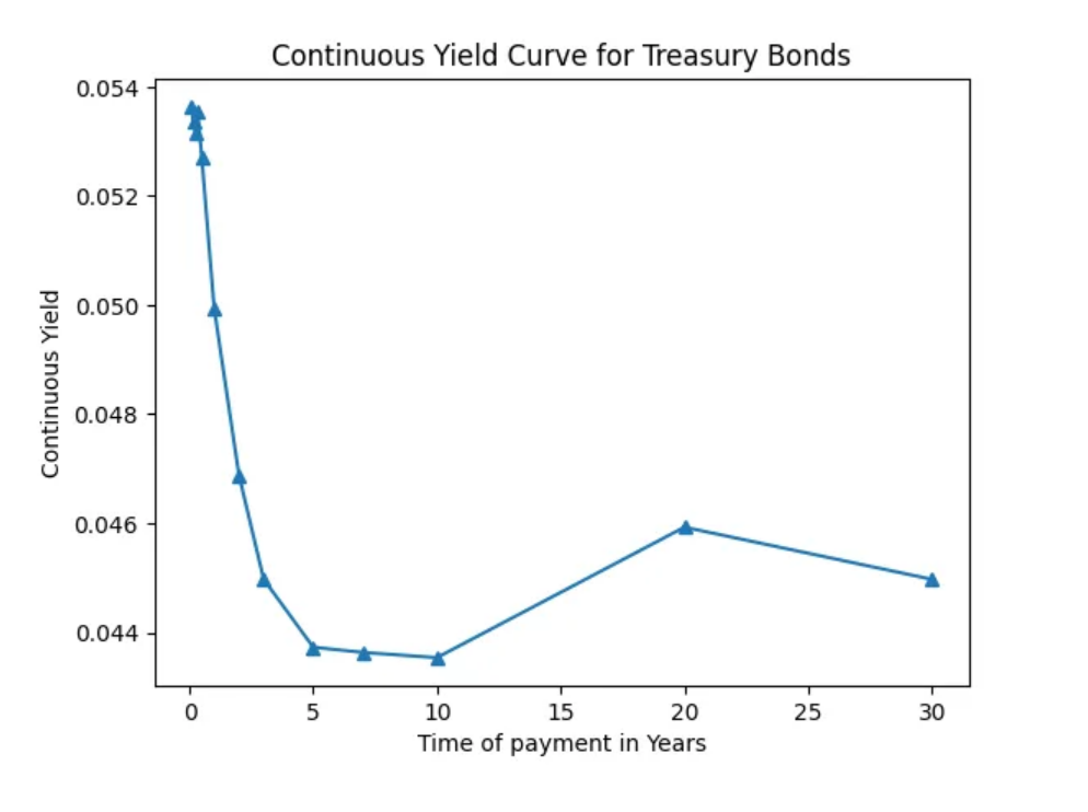
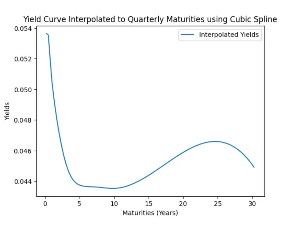
The next step is to convert the par yields to a continuous rate, simplifying calculations by making it easier to discount future cash flows. Since our bond pays coupons quarterly, we must also determine the appropriate discount factor that aligns with these periodic payments. To accomplish this, we convert the yield curve to a continuous yield curve and then interpolate this curve, creating a smoothed yield curve that provides discounted values for each quarter over the 30-year term.
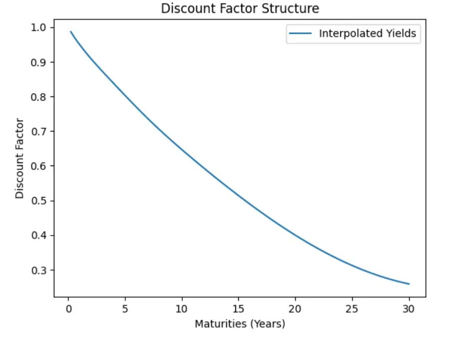
Now that we have our interpolated yield curve we can use the new yields and multiply by the period to get the present value of our cash flows. Shown below is our discount factor, as we go out further in time with our payments the value of those payments should go down since a dollar is worth today rather than getting a dollar one year from now.
Now, let’s delve into the bond calculations, starting with the present value. Present value represents the total value of all future cash flows discounted to today’s terms. For our bond example, the present value is 370.45.
Yield to maturity (YTM) is the total return on investment if we hold the bond until maturity and receive all cash payments. The YTM can be calculated using the following formula
PV = (∑C(e^-yt)) + F(e^-yt)
Where:
For this bond, the YTM is 0.1997. If we hold this bond until the end of its last payments, we receive a 19.97% return on our investment.
For this bond, the YTM is 0.1997. If we hold this bond until the end of its last payments, we receive a 19.97% return on our investment.
Next, we consider the bond’s duration, for this example, we are using the modified duration which measures how the bond’s value changes in response to a 100 basis point (1%) change in interest rates. This is important because we need to see how sensitive our bonds change due to interest rates. The formula for our duration calculation is below.
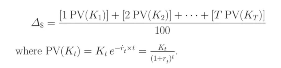
Where:
For our bond, the duration is 5.1959, meaning that if interest rates increase by 1%, the bond’s price will decrease by 5.1959%.
Finally, convexity measures the curvature in the bond’s price-yield relationship and represents the rate of change of duration. This helps us better understand how the bond price changes, particularly in response to large interest rate movements, and explains why prices tend to increase more when yields fall than they decrease when yields rise by the same amount. The formula for convexity is presented below.
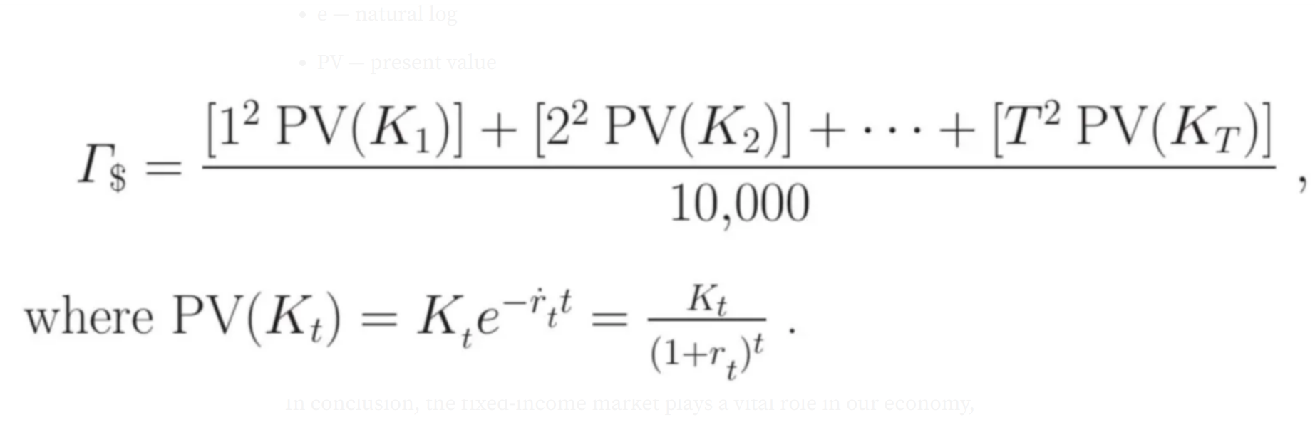
For our example, the bond’s convexity is .5122. So this means that if yields were to change by 1% the adjusted duration price estimate would change by .5122.
In conclusion, the fixed-income market plays a vital role in our economy, offering valuable insights into the pricing of a company’s debt. Using continuous yields provides flexibility in bond pricing while interpolating these yields to estimate the value of bonds with various maturities and coupon payments. Furthermore, by combining duration with convexity, we can gain a more comprehensive understanding of how changes in interest rates impact bond pricing, allowing for more informed investment decisions.
Can code be found here
https://github.com/Gaiden-Spence/Basic-Bond-Analytics-